Research
Our work runs along a single axis: from characterization to modelling. Laboratory tests and field measurement establish how rock and rock masses actually behave; those observations are then turned into computable models; and numerical simulation finally answers the engineering and hazard questions.
Rock is a natural material, and its mechanical behaviour differs greatly from that of the man-made materials we usually deal with. At the microscopic scale the arrangement of mineral grains governs how cracks develop under load; at the macroscopic scale the distribution of joints governs stability and engineering behaviour. Understanding that behaviour is the core objective of this laboratory.
CharacterizationModelling
Rock Testing
The greatest difference between rock and other materials is that rock usually sits under high confining pressure, where its behaviour is quite unlike that at low confinement: strength rises markedly and the material turns from brittle to ductile. The triaxial system is therefore the central instrument of rock mechanics. Ours is a GCTS RTX-1000, used for uniaxial, triaxial and indirect tensile (Brazilian) tests, with a maximum load of 1000 kN and a maximum confining pressure of 70 MPa.
Beyond strength and deformability, results from several confining pressures are combined into failure criteria that feed the numerical models downstream.
More recently we added acoustic emission measurement: the elastic waves released as micro-cracks initiate and propagate are recorded during loading, so failure can be followed as a process rather than reduced to a single peak value. For the weak rocks common in Taiwan we also use the needle penetration test as a simple strength index.
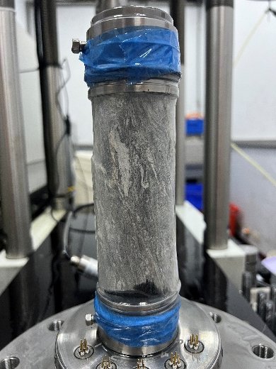 Triaxial specimen
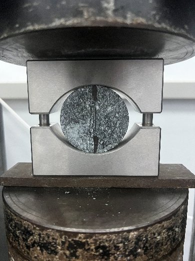 Brazilian (indirect tensile) test
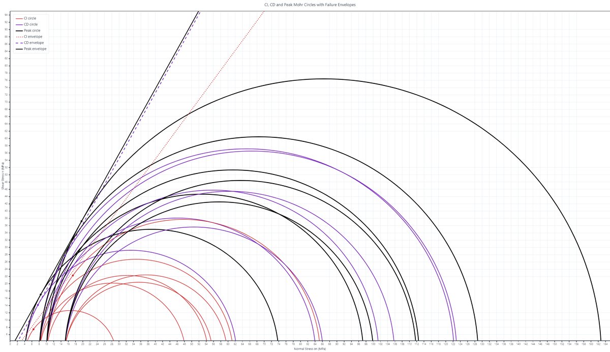 Failure criteria from several confining pressures
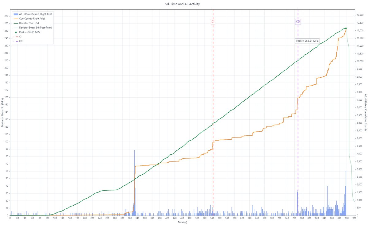 Acoustic emission against load history
Point Cloud Analysis
Field investigation is the first step towards understanding a site, and traditionally the most labour-intensive, the slowest and the most subjective. We build three-dimensional point clouds of outcrops by photogrammetry and LiDAR, then extract joint orientation, roughness and fracture traces algorithmically — turning field measurement into something quantitative and repeatable.
Current work covers outcrop characterization (joint sets, orientation distributions, JRC roughness statistics), fracture extraction and discrete fracture network construction, and a semi-automatic rock mass rating program that derives a Q-system score directly from the point cloud rather than from item-by-item engineering judgement.
We also collect engineering geological data from across Taiwan, compiling the mechanical properties of rock materials and joint surfaces into a database that design and construction organisations can use as a first reference.
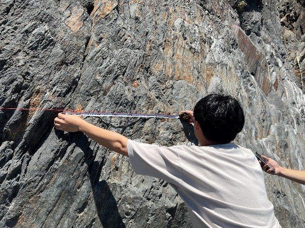 Joint measurement in the field
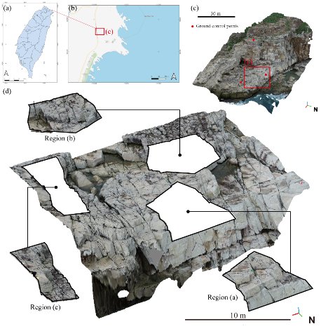 Outcrop model from photogrammetry
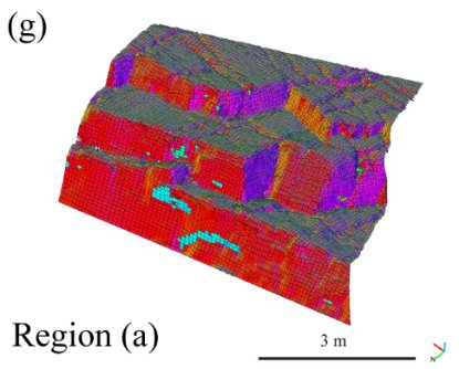 Automatic point cloud clustering
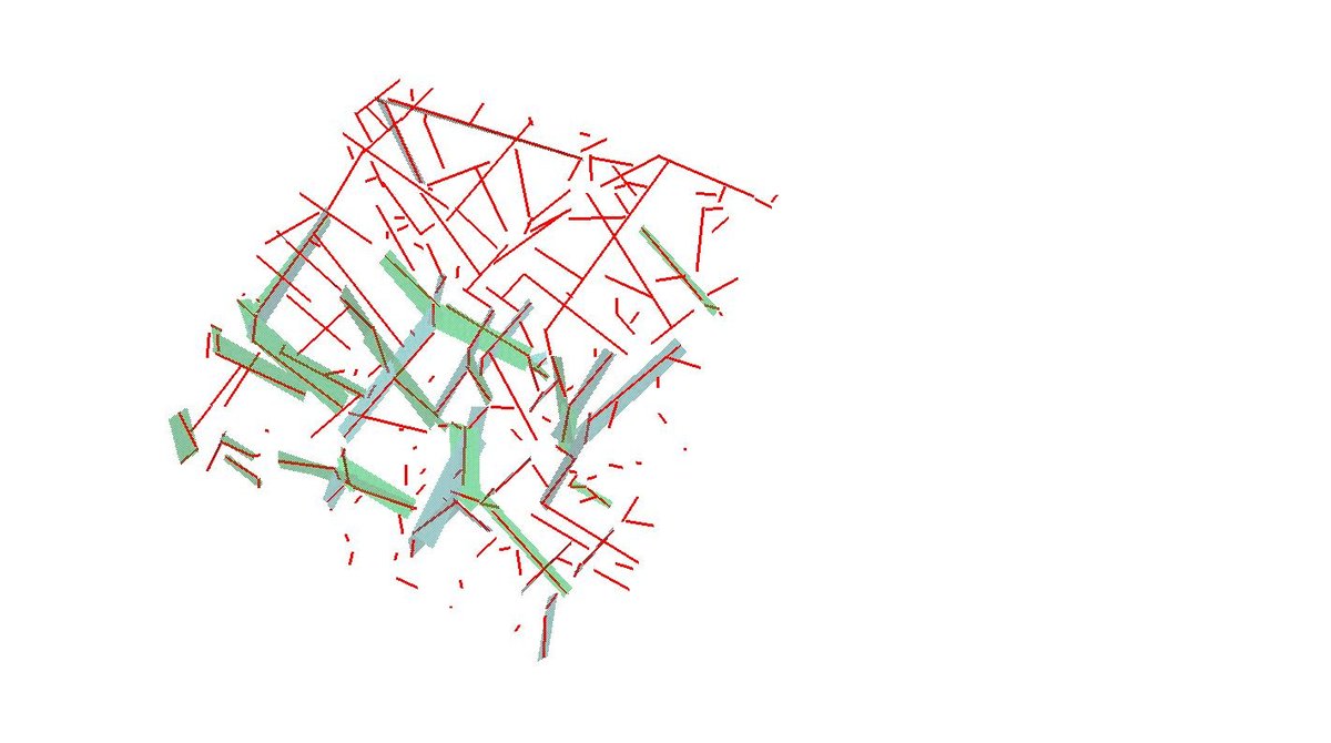 Fracture extraction and DFN
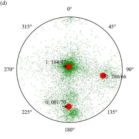 Joint orientation distribution
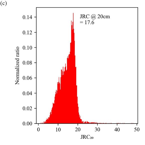 JRC roughness statistics
Consumer-Grade LiDAR Monitoring
High-end LiDAR is expensive and bulky, which makes long-term deployment impractical. We are investigating whether consumer-grade LiDAR — the kind built into mobile devices — is accurate enough for displacement monitoring: laboratory tests establish its error characteristics and the smallest detectable movement, long-term field monitoring validates it, and the influence of temperature and rainfall is analysed.
If it works, the cost of monitoring slopes and retaining structures over long periods drops sharply.
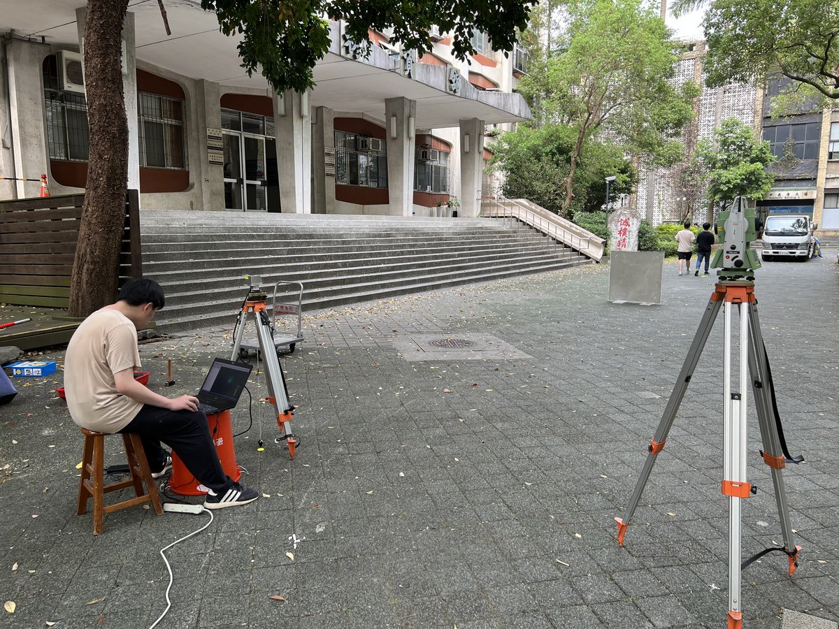 Field deployment and scanning
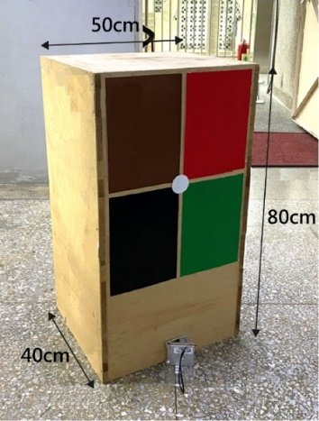 Laboratory displacement validation
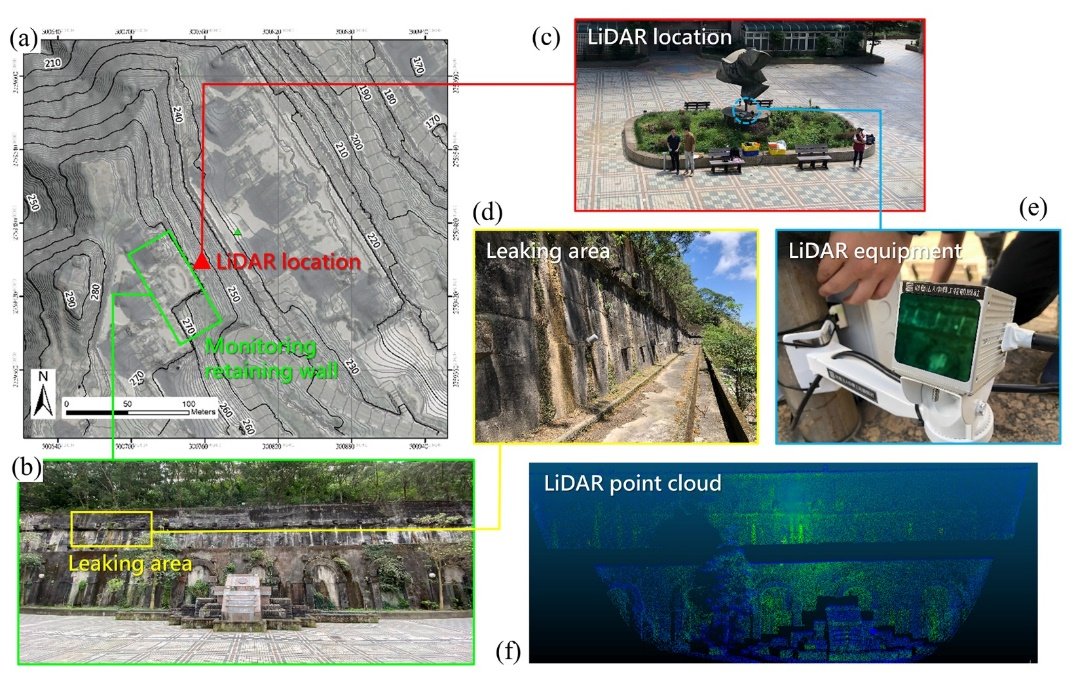 Long-term monitoring of a retaining wall
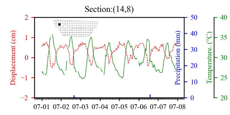 Displacement against temperature and rainfall
Model Development
The discrete element method (DEM) was proposed by Cundall in 1971. It computes the motion of elements through a force–displacement relationship, reproducing macroscopic response from the interaction between particles, and — depending on whether bonds are introduced — can represent both continuous and discrete bodies.
Generic DEM contact models, however, rarely reflect how rock actually behaves. Our work is to turn laboratory and field observation into contact models the method can compute; this is where the laboratory’s main academic contribution lies.
Particulate Interface Model (PIM)
An “interface” here means any contact surface between solids, not only geological weak planes such as joints or cleavage. In rock engineering the mechanical properties of interfaces govern the stability of the rock mass. The most advanced interface model available in DEM, the smooth joint model, does not account for the geometrical arrangement of particles during shearing, and so cannot reproduce interface behaviour accurately.
By considering the contact and separation of a group of particles under shear, introducing several corrections, and incorporating the two failure criteria most used in practice — Mohr–Coulomb and Barton–Bandis — we developed the Particulate Interface Model. Its input parameters can be taken straight from laboratory data without back-calculation, and it removes the dependence of the result on particle size.
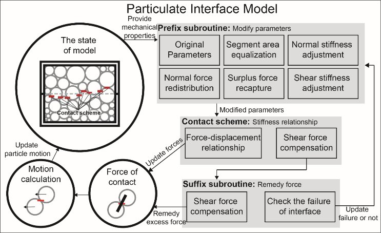 Computation scheme of the model
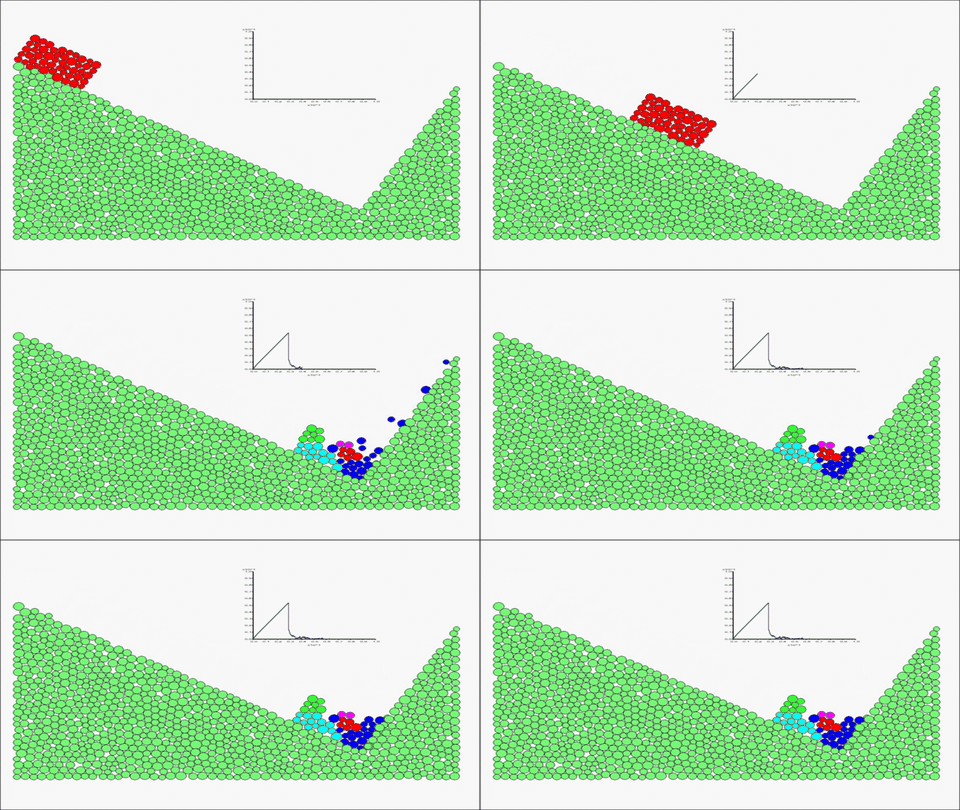 Planar sliding with velocity-dependent friction
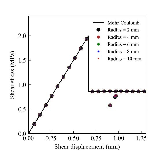 Consistent results across particle sizes
Seepage Model
Water in a rock mass drives many engineering failures. We built a fracture seepage model within DEM in which the pore space between particles forms the flow path, extended it to three dimensions, and use it to study the hydrogeological behaviour of jointed rock masses and hydro-mechanical coupling.
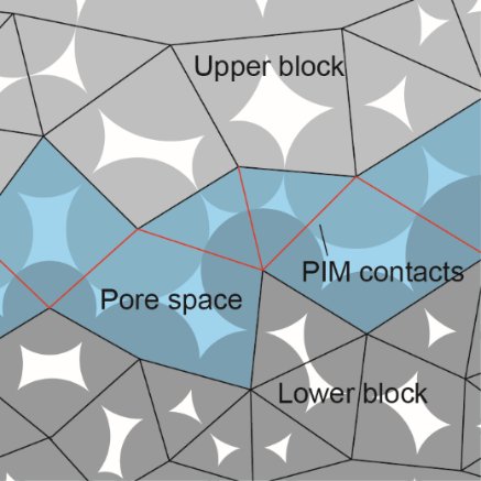 Pore space and interface contacts
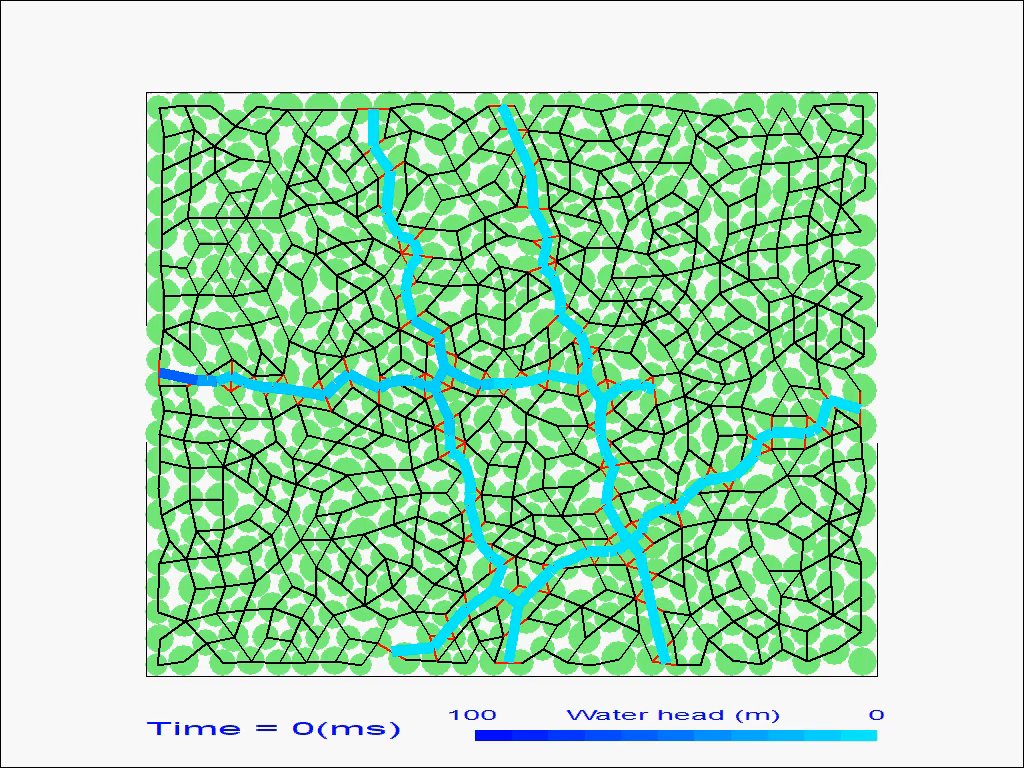 Two-dimensional fracture seepage
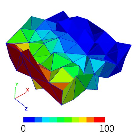 Three-dimensional head distribution
Biconcave Bond Model
Unlike soil, rock has considerable cohesion, and the cementation between grains governs its mechanical behaviour. Examining thin sections we found the cement between grains approximates a biconcave shape, and from that developed the Biconcave Bond Model together with the corresponding DEM contact algorithm.
When specimens of known geometry and fabric are simulated, the micro-scale parameters the model requires lie closer to the values measured in the laboratory — so predicting macroscopic behaviour from micro-scale parameters works better.
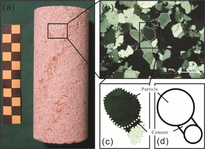 Grains and cement in thin section
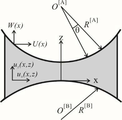 Biconcave cement geometry
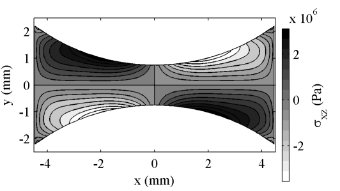 Stress distribution within the cement
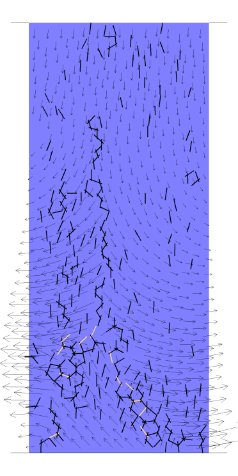 Simulated crack development
Gravel Deposit Modelling
Gravel deposits are widespread in the foothills of western Taiwan. They are neither soil nor intact rock: a mixture of blocks of widely varying size in a fine matrix, whose behaviour is governed by the shape and arrangement of the blocks. Generic models that approximate particles as spheres cannot reproduce the real interaction and interlocking between them.
We scan actual blocks and rebuild them as numerical models that preserve their geometry, then use those to simulate triaxial and in-situ direct shear tests and examine how block content, shape and arrangement affect overall strength.
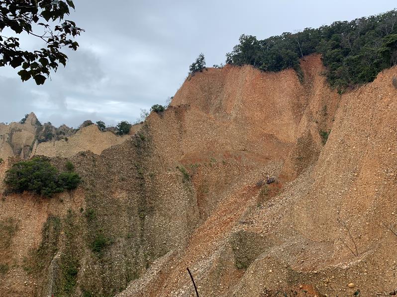 Gravel deposit outcrop
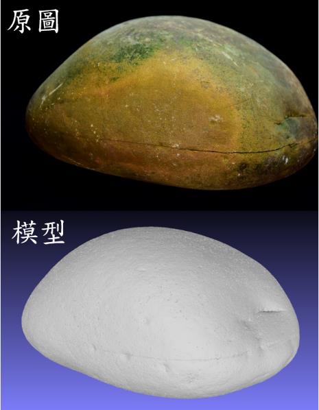 A block and its reconstructed model
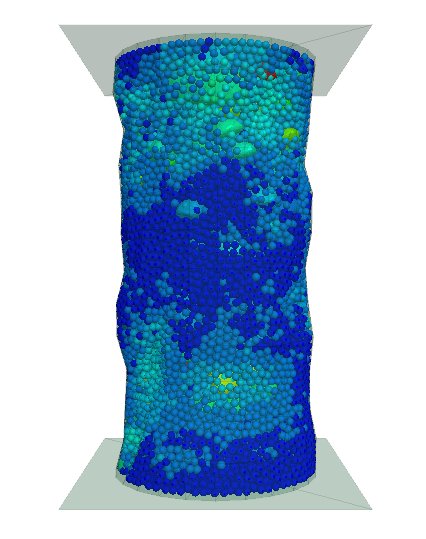 Specimen simulation with block geometry
Jointed Rock Mass Simulation
We tend to assume the rock around a geotechnical work is a homogeneous, isotropic foundation. That holds for an intact block or a heavily fractured mass, but once one or more joint sets are present the strength and deformability vary with direction and the behaviour becomes highly complex. Jointed rock masses are therefore one of the principal challenges of rock mass engineering.
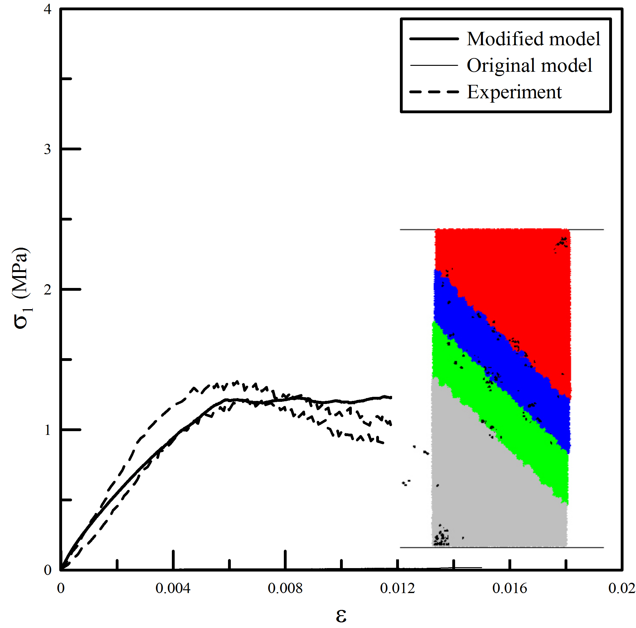 Jointed rock mass specimen
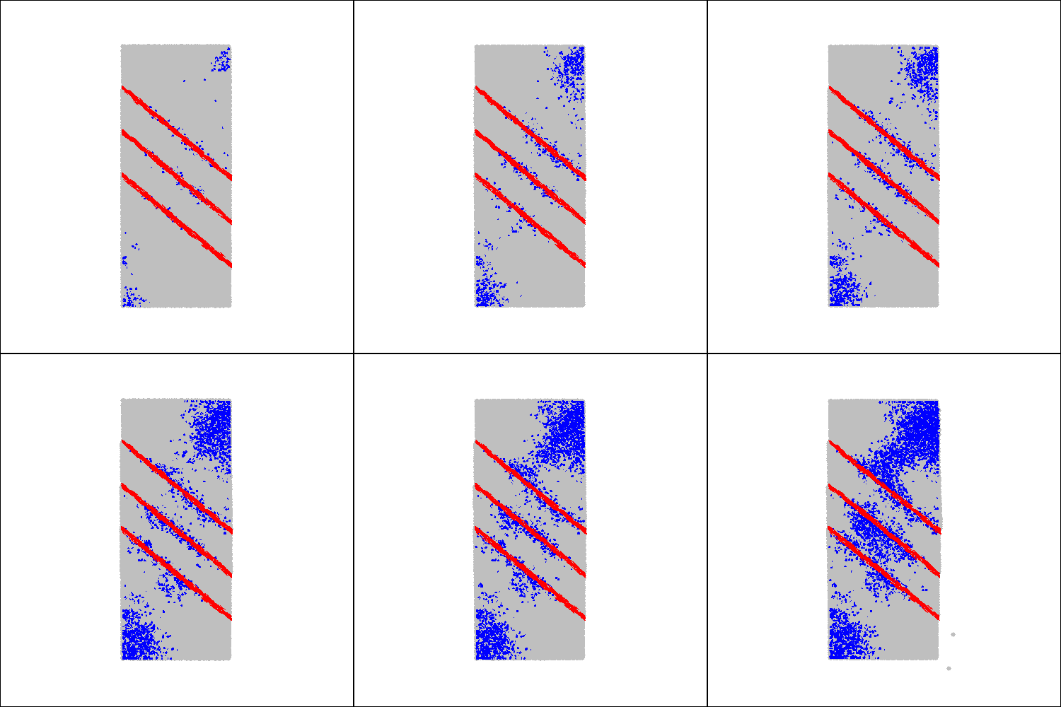 Crack development under loading
Numerical Simulation
The last step is to apply those models to real cases: reproducing how a hazard developed, and supporting the authorities in their assessment and decisions.
We took part in the investigation and analysis of the Highway No. 7 49.8K landslide, covering rockfall simulation, debris flow and its interaction with a bridge, and estimation of the run-out after failure. This kind of work is collaborative — microseismic technique from NYCU, multiscale field survey from NTU and Sinotech, with this laboratory responsible for the discrete element modelling.
As development demands grow, designs become more complex and conventional calculation no longer suffices. Numerical analysis both examines the safety of a design in advance and reconstructs what happened after a failure.
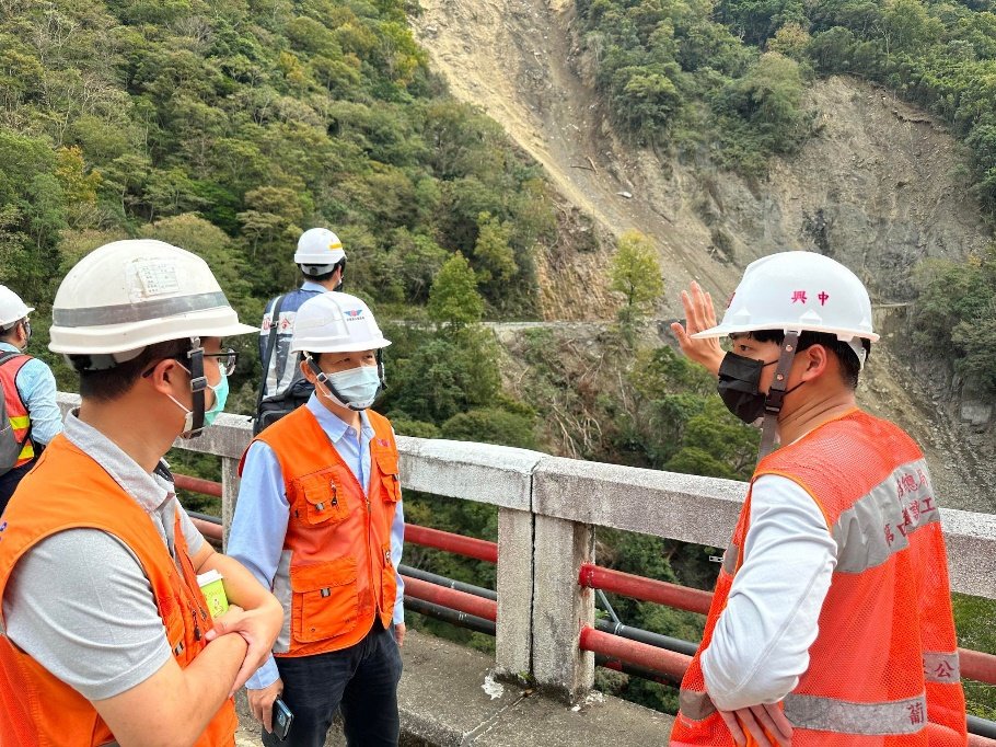 Site investigation at Highway No. 7 49.8K
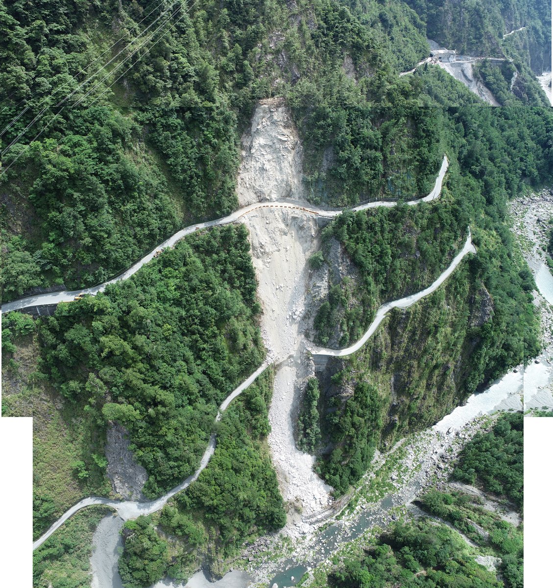 Aerial view of the failure
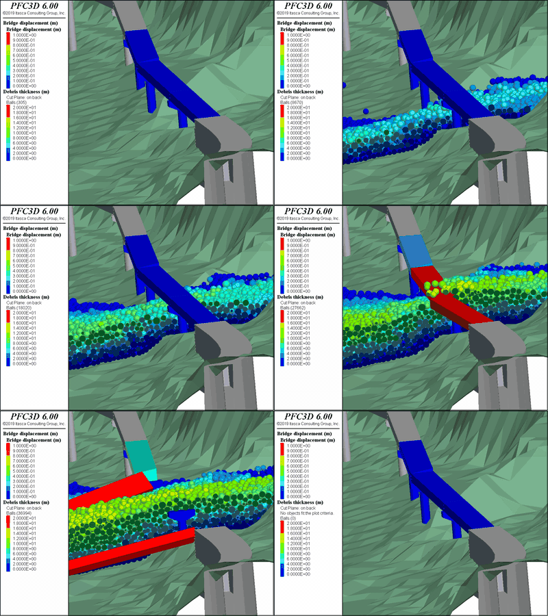 Debris flow interacting with a bridge
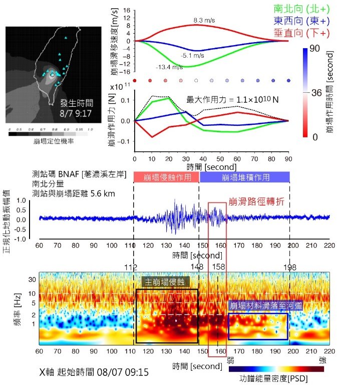 Microseismic signal analysis (NYCU)
Excavation Damaged Zone
After a tunnel is excavated the surrounding rock is damaged by the redistribution of stress, forming a ring known as the excavation damaged zone (EDZ). Its extent and the change in permeability across it determine both the long-term stability of the tunnel and the containment of a geological disposal facility.
We track the displacement developing at each excavation stage and the extent of the damaged zone using discrete and continuum analysis, extending the time scale from construction out to tens of thousands of years to assess how the zone evolves.
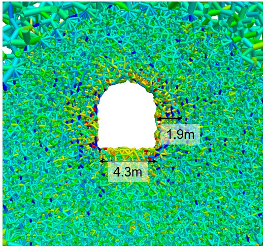 Extent of the damaged zone after excavation
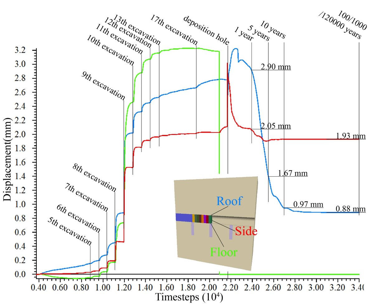 Displacement from excavation to the long term
Applications
All of this points back to the practice of geotechnical and resources engineering. Foundation excavation, slope stability, dam analysis, tunnelling, the investigation and remediation of landslides — every one of them is bound up with people’s daily lives. Every piece of construction has its foundation laid by geotechnical engineering: before Taipei 101 could rise, its piles had to be driven; before the high speed railway could be built, slopes had to be stabilised and tunnels excavated.
Taiwan is a place well worth exploring for this field. A small island holds structures and lithologies of every kind; its stone industry is advanced in both quarrying and processing; and because the geology is young and fragile, with severe rainfall and earthquakes, the demand for specialists in geotechnical engineering and hazard mitigation is very large.
 Tunnel construction site